
Comparing development experience and runtime efficiency of dbt and SQLMesh.
dbt has played a significant role in simplifying the onboarding process for teams of data analysts looking to automate data transformation and standardize business logic.
However, as data teams manage larger and more complex projects consuming greater quantities of data, they begin to encounter challenges that outpace dbt’s capabilities. To address these limitations, new dbt features have been gradually added and developers have built out an impressive open-source ecosystem of dbt packages. Nevertheless, this expansion often introduced increased complexity and risks, stemming from the simplistic nature of the product’s foundation.
In this post, I offer a side by side comparison of what the development process looks like when using dbt (both basic and advanced modes of operation) vs using SQLMesh. I demonstrate how user’s don’t have to choose between simplicity and efficiency.
The comparison aims to cover two aspects of the process: the user experience and the runtime efficiency. To make the comparison independent from any particular data warehousing technology, the runtime efficiency will be measured in numbers of model executions.
Setup
The comparison is made using a theoretical project setup which consists of 50 models.
Each subject in this comparison is evaluated using the following process which reflects a typical data transformation development workflow:
- Make a change within the project
- Deploy the change to the development environment for validation and review
- Deploy the change to the production environment once it passes validation
The following constraints and conditions apply when making a change:
- The change impacts 3 models directly. In other words, the definition of 3 models changed in some way.
- The change indirectly impacts 10 downstream models. Even though their definitions didn’t change, they may still need to be re-executed to prevent possible regressions.
- The 3 directly impacted models rely on input from 10 upstream models.

For the sake of cost and runtime efficiency, I assume that impacted models run incrementally, processing only previously unseen rows on each execution. If you are not familiar with incremental load patterns, my colleague Toby Mao explains the concept well in his post.

dbt
In this section I describe different modes of operation of dbt that have been selected for this comparison.
dbt run
This mode of operation relies on the plain dbt run command without any extra configuration. It is the simplest approach when using dbt, but also the most runtime inefficient one.
For simplicity’s sake, I assume that the development environment has already been provisioned (e.g. a separate database has been created) and the corresponding target is available. Typically, provisioning the development environment requires additional steps and configuration.
Remember that one of the requirements is for tables in the development environment to accurately reflect their counterparts in production. To achieve this the following command is required to prepare the development environment and populate it with data:
$ dbt run --target dev --full-refresh
This command executes all 50 models in the development environment.
Once the change to the 3 models has been reviewed and approved, we are ready to deploy to production. The same command is run again but against the production target.
$ dbt run --target prod --full-refresh
Consequently, all models are re-executed, this time in the production environment.

Despite its seeming simplicity, this naive approach results in significant runtime overhead with 100 model executions total. Fortunately dbt offers additional tools to mitigate this.
dbt run with selection
The extension of the previous approach is to use node selection syntax as part of the dbt run command.
With this approach all impacted models and models that provide input (23 models total) should be selected as part of the run command. Thus, the development environment can be populated as follows:
$ dbt run --target dev --full-refresh --select \
        +directly_modified_model_one+          \
        +directly_modified_model_two+          \
        +directly_modified_model_three+
Plus signs in the command above inform dbt that we want to also include models that are upstream and downstream from the specified ones. This command can be simplified through the use of tags and / or selectors as long as the user is confident that all relevant models will be included. dbt will not notify the user in any way if the latter is not the case.
When deploying to production the same command is used with the --target argument set to prod and leading “+” signs removed to exclude upstream models from the execution:
$ dbt run --target prod --full-refresh --select \
        directly_modified_model_one+            \
        directly_modified_model_two+            \
        directly_modified_model_three+
This approach is a significant improvement over the previous one with 36 model executions total:
- 6 executions of directly modified models (3 in dev & prod respectively)
- 20 executions of indirectly modified models (10 in dev & prod respectively)
- 10 executions of models that provide input (10 in dev only)
dbt run with deferral
Another optimization that can be made is reusing the input data from the production environment in the development environment. This eliminates the need for executing models that produce this input data.
dbt offers the deferral functionality to achieve exactly this. Note that it’s explicitly stated in the documentation that using this feature is not trivial and requires careful consideration.
With this approach, the command from the previous section no longer needs to include input models. Instead it requires a path to the manifest from a previous dbt invocation on production:
$ dbt run --target dev --full-refresh --select state:modified+ \
        --defer --state /path/to/state
When deploying to production the same command is used with the --target argument set to prod.
This approach brings down the number of required executions to 26, but imposes additional burden on a user to generate, store, and select the right state file during each development cycle.
Furthermore, if the user's local state doesn't match the one provided in the manifest file, the tool silently recomputes the entire graph, thereby defeating the purpose of this optimization.
As a result, this approach is the most complex and error-prone among the options compared, as the tool does not make any attempts to rectify any mistakes made by the user or help them manage the state.
Custom tools and scripts
It’s worth pointing out that dbt can be enhanced with vendor-specific features provided by the underlying cloud data provider.
The example of this is zero-copy clones in Snowflake or analogous features from other providers.
Such cases are excluded from this comparison for several reasons:
- The specific implementation details and constraints of such features vary greatly among different cloud providers. This comparison is intended to be vendor-agnostic.
- These features are not a part of the dbt product offering and require custom automation tooling and / or complex manual steps.
Summary
dbt offers a variety of solutions for optimizing runtime efficiency and reducing the cost. It is clear, however, that as the runtime efficiency increases, the complexity of using these solutions, as well as their proneness to errors, grows proportionally.

SQLMesh
Every time users need to apply changes to any environment in SQLMesh they use the sqlmesh plan command. The command for the development environment looks as follows:
$ sqlmesh plan dev
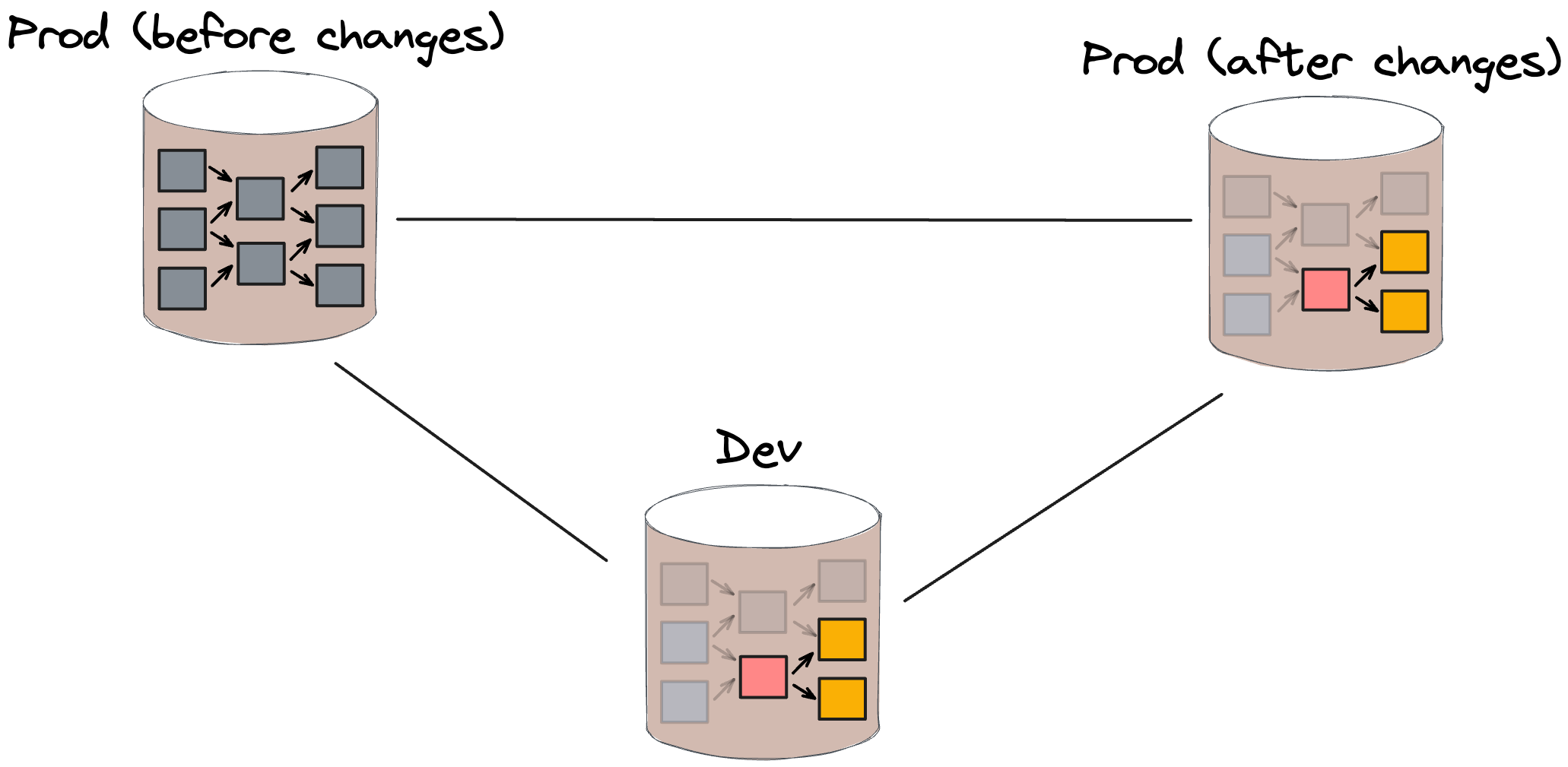
The command above automatically creates the dev environment if it doesn’t exist. The new environment is automatically populated with data from production without requiring any additional computation. The tool guarantees that all changes made to this environment are completely isolated and don’t impact other environments.
SQLMesh tracks the state of each model and can automatically determine which models have been changed either directly or indirectly. Only impacted models are executed as part of the development environment while data from other models is safely reused from production. This is similar to dbt’s deferral feature but without any user involvement or state management.
After code review and once changes are ready to be deployed to production, the same command is used with the prod argument:
$ sqlmesh plan prod
SQLMesh guarantees the absence of data gaps in all modified tables, enabling their secure reuse in the production environment. This eliminates the need for an additional round of model executions, bringing the total number of model executions down to 13:
- 3 executions of directly modified models in dev only
- 10 executions of indirectly modified models in dev only

This improvement is made possible through the implementation of a technique called Virtual Data Environments within SQLMesh. Adam Stone wrote an excellent post about it.

As a bonus, the chart above also includes an additional case in which changes applied to the 3 models have no actual downstream impact. In this case, SQLMesh can automatically identify the non-breaking nature of these changes and reduce the number of required model executions down to just 3.

Final Thoughts
Developing models using dbt’s default mode of operation, may result in significant runtime cost. dbt mitigates this by offering various ways of manually defining what gets executed in order to reduce runtime costs. However, when considering the user experience, the level of complexity in utilizing dbt increases in direct correlation with the desired level of runtime efficiency. As the number of model executions decreases, the developer process becomes more intricate, involved and error-prone.
SQLMesh, on the other hand, automates the complexity away, lifting the burden from the user, while maximizing the runtime efficiency as much as possible through the elimination of redundant model executions. Your data team can get back to doing what they do best: defining data transformations and deploying trustworthy models without the fuss.
I hope this comparison will help you make informed decisions around increasing productivity and optimizing runtime efficiency within your organization. Join our Slack community to connect with other data practitioners who face similar challenges.


