
Writing efficient and correct incremental pipelines is challenging. While many folks do take on the challenge of writing incremental models, it is viewed as an advanced use case which could discourage teams from adopting incremental loads.
Writing efficient and correct incremental pipelines is challenging. While many folks do take on the challenge of writing incremental models, it is viewed as an advanced use case which could discourage teams from adopting incremental loads.
When working with large fact/event tables, like tracking sessions or impressions, it may take too long or be too expensive to recompute the entire history every run. When I worked on the video streaming data team at Netflix, I regularly worked on pipelines that had to churn through terabytes of new data daily. It would have been impossible to process these pipelines from scratch every day.
In this post, I’m hoping to demystify incremental loads. I’ll walk through a couple techniques for loading incrementally and some advanced use cases and considerations. Even if you aren’t processing terabytes of data, data pipelines could become much more efficient, saving you time and money.
Reading data incrementally
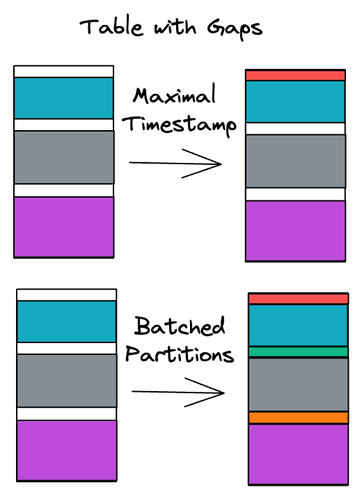
There are two main ways to read data incrementally: maximal timestamp (popularized by dbt) and date partitions (popularized by Airflow / Hive).
Maximal timestamp
Reading data by finding the maximal timestamp is a two-step approach:
- If the table doesn’t exist, compute the whole history in one shot
- If the table does exist, query it to find the last processed timestamp and then use that to filter the upstream source data.
An example query looks like this:
SELECT *
FROM raw.sessions
{% if is_incremental() %}
WHERE ts > (SELECT MAX(ts) FROM {{ this }})
{% endif %}
The main benefits of this approach is that it doesn’t require extra state besides what’s stored in the table. However, it has drawbacks especially when operating at scale.
- It assumes that you’re able to load the entire table in one go. At large scales, processing large fact tables may require batching (eg. 1 month chunks) in order to reliably complete.
- The query is more complicated to write and maintain because there are two modes of operation, one for the initial load and one for incremental.
- Custom SQL is often needed to handle incremental models differently in development in order to enable faster testing and validation, eg. only computing 1 day of data.
- You cannot detect or fix data gaps that may occur due to custom scripts or the addition of historical data.

Date Partitions
When writing pipelines for scheduler based systems, like Airflow, the scheduler provides a run date which you can base your query on. When backfilling, these dates can be overridden to the backfill range.
SELECT *
FROM raw.sessions
WHERE ts BETWEEN {{ start }} AND {{ end }}
The main drawback of this approach is that extra state is needed in order to understand which intervals have been processed, but this is usually stored and managed by the scheduler (like Airflow).
However, there are many advantages to this approach compared to maximal timestamps.
- The queries are simpler because there’s only one mode of operation (no incremental vs full load).
- Backfills are more scalable and reliable because they can be easily batched up into manageable chunks.
- You can easily compute just one day of data or manually fix gaps by overriding start and end.
Writing data incrementally
There are two main ways to make your incremental pipeline idempotent even with late arriving data: merge and insert overwrite. Idempotency is the property that running the same query twice with the same inputs results in the same output. Loading data with the append strategy is an example of a non idempotent pipeline. If you accidentally run it twice on the same data, you’ll end up with duplicates.
Merge
Merge is a newer technique and works by matching rows between a source and target on a key, and then updating or inserting it.
MERGE processed.sessions t
USING raw.sessions s
ON t.uuid = s.uuid
WHEN MATCHED THEN UPDATE SET …
WHEN NOT MATCHED THEN INSERT …
As long as there is a primary key or set of keys to join on, merge is a great way to ensure your data is consistent and prevent duplicate rows. You can specify your logic to insert data when it doesn’t exist and update it when it does.
Insert overwrite
At Netflix, we used insert overwrite, which is a technique popularized by Hive and carries over to Spark / Databricks. These systems use partitions which are essentially folders containing groups of data. In incremental systems, you’ll usually have one folder per day. Insert overwrite will atomically delete a folder before writing contents into it, ensuring idempotency.
INSERT OVERWRITE TABLE processed.sessions
PARTITION(ds=...)
SELECT …
This approach requires that you provide the full data for each partition you are writing.
Comparison
Merge can be inefficient if partition pruning is not passed into the predicate. This is because in order to ensure that there are no duplicates, the engine must join all existing records with all new records to ensure uniqueness.
Merge is extremely efficient when only a few records need to be updated (like removing one or two records for GDPR) because it minimizes the need to rewrite files. However when processing late arriving data, there are usually many records that need updating and so there isn’t a clear efficiency benefit of using merge over insert overwrite.
Conversely, insert overwrite is inefficient when only a few rows have changed because it has to completely rewrite all files of a partition. However, in this case, because many files need to be touched anyways, insert overwrite doesn’t have to pay the cost of ensuring all rows are matched.
Dealing With Late Arriving Data
Events can arrive much later than when they were triggered. For example, you can watch downloaded shows on Netflix even without an internet connection. These sessions only get synced when the device comes back online. Late arriving data can be tricky to handle and requires special handling. In general, most events are received close to when they were triggered, so a reasonable threshold (like 14 days) can usually catch 99% of events.
Reading late arriving data
In order to capture late arriving data, you can simply subtract a window of time that you’re comfortable with.
Reading with maximal timestamp
SELECT *
FROM raw.sessions
{% if is_incremental() %}
WHERE ts > (SELECT MAX(ts) FROM {{ this }}) - 14
{% endif %}
Reading with date partitions
SELECT *
FROM raw.sessions
WHERE ts BETWEEN {{ start  - 14}} AND {{ end }}
Writing late arriving data
However, when an incremental pipeline "looks back", it processes data that has already been seen. If done naively, this could cause your pipelines to contain duplicates, which is not acceptable!
In order to efficiently and correctly handle look backs, your pipelines should define the expected range of outputs. You can filter your resulting dataset to only the range that you expect to write. For example, you may read data that is a year old, but you should drop it as it’s not within your expected tolerance.
When using merge, you should push this expected range down to the merge so you’re not doing a full scan of all historical uuids. With insert overwrite, you need to read in all previous rows in the expected range so you don’t lose historical records.
Conclusion
Incrementally loading data is one of the most cost effective ways to scale your warehouse. When done correctly, you can save money, time, and increase the reliability of your systems.
Join our Slack Channel to chat more about scalable data infrastructure. Check out SQLMesh which makes writing incremental computation easy and safe.


